原文地址:
https://pytorch.org/tutorials/beginner/blitz/neural_networks_tutorial.html
NEURAL NETWORKS 【神经网络】
可以使用torch.nn包来构建神经网络。
现在您已经了解了autograd, nn依赖autograd来定义模型并区分它们。一个nn.Module包含层,和一种方法forward(input),它返回output。
例如,对数字图像的分类网络:
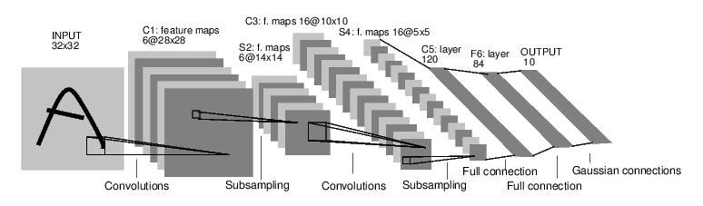
卷积神经网络
它是一个简单的前馈网络。它获取输入,一个接一个地通过几个层,最后给出输出结果。
神经网络的典型训练过程如下:
- 定义具有一些可学习参数(或权重)的神经网络
- 迭代输入数据
- 通过网络处理输入
- 计算损失(输出与正确结果的距离)
- 将梯度传播回网络参数中
- 更新网络中的权重,使用简单的典型的更新规则:weight = weight - learning_rate * gradient
定义网络
让我们定义这个网络:
1 | import torch |
输出:
1 | Net( |
你仅仅只需要定义forward函数,并且使用autograd会自动帮你定义backward函数(计算梯度的地方)。你可以在forward函数中使用任何Tensor操作。
模型的可学习参数由net.parameters()返回
1 |
|
输出
1 | 10 |
让我们尝试一个随机的32x32输入注意:这个网络(LeNet)的预期输入大小是32x32。要在MNIST数据集中使用这个网络,请将数据集中的图像调整到32x32。
1 | input = torch.randn(1, 1, 32, 32) |
输出
1 | tensor([[ 0.0435, -0.1141, -0.0298, -0.0904, 0.1214, 0.1464, -0.0767, 0.0372, |
使用随机梯度将所有参数和反向传播的梯度缓冲区归零:
1 | net.zero_grad() |
注:
torch.nn只支持小批量。整个torch.nn包只支持小批量的样本输入,而不是一个单一的样本。
例如:nn.Conv2d将使用4D的tensor nSamples x nChannels x Height x Width.
如果你只有一个单一样本,只需要使用input.unsqueeze(0)去添加一个假的批处理维度。
在继续之前,让我们回顾一下到目前为止您所看到的所有类。
概要:
- torch.tensor 支持例如backward()的autograd操作的多维数组。也保留了tensor的梯度。
- nn.Module 神经网络模型。使用帮助成像将它们移动到GPU,输出,加载等,方便的封装参数。
- nn.Parameter Tensor的一种,当分配一个属性给Module的时候,会自动注册一个参数。
- autograd.Function 实现autograd操作的前向和后向定义。每一个Tensor操作,至少创建一个Function节点,该节点连接到一个创建的Tensor并且对它的历史编码。
在这点上,我们覆盖包含了:
- 定义了神经网络
- 处理输入并且向后调用
还剩下:
- 计算损失
- 更新神经网络的权重
损失函数
损失函数使用一对输入(输出,目标),并且计算一个值来估计输出到目标的距离。
在nn包下有几种不同的损失函数。一个简单的损失是:nn.MSELoss它计算输入和目标之间的均方误差。
例如:1
2
3
4
5
6
7output = net(input)
target = torch.randn(10) # a dummy target, for example
target = target.view(1, -1) # make it the same shape as output
criterion = nn.MSELoss()
loss = criterion(output, target)
print(loss)
输出:1
tensor(1.1380, grad_fn=<MseLossBackward>)
现在,如果您按照loss向后方向,使用其 .grad_fn属性,您将看到如下所示的计算图:
1 | input -> conv2d -> relu -> maxpool2d -> conv2d -> relu -> maxpool2d |
因此,当我们调用时loss.backward(),整个图形会随着损失而区分,并且图形中的所有张量都requires_grad=True 将.grad使用渐变累积其Tensor。
为了说明,让我们向后退几步:
1 | print(loss.grad_fn) # MSELoss |
输出:1
2
3<MseLossBackward object at 0x00000225B8275CF8>
<ThAddmmBackward object at 0x00000225B8275DA0>
<ExpandBackward object at 0x00000225B8275CF8>
BACKPROP 【反向传播】
要反向传播错误,我们所要做的就是loss.backward()。您需要清除现有渐变,否则渐变将累积到现有渐变。
现在我们就调用loss.backward(),看一下conv1在向后之前和之后的偏差梯度。
1 | net.zero_grad() # zeroes the gradient buffers of all parameters |
输出:
1 | conv1.bias.grad before backward |
现在,我们已经看到了如何使用损失函数。
唯一要学习的是:
- 更新网络权重
更新权重
实践中使用的最简单的更新规则是随机梯度下降(SGD):
weight = weight - learning_rate * gradient
我们可以使用简单的python代码实现它:
1 | learning_rate = 0.01 |
但是,当您使用神经网络时,您希望使用各种不同的更新规则,例如SGD,Nesterov-SGD,Adam,RMSProp等。为了实现这一点,我们构建了一个小包:torch.optim它实现了所有这些方法。使用它非常简单:
1 | import torch.optim as optim |
注意:
观察如何使用optimizer.zero_grad()手动将梯度缓冲区设置为零。这是因为梯度是按照Backprop部分解释的那样积累的。